Managing Relationships in Power BI

When creating reports in Power BI, you will typically create a data model that has several tables. To provide meaningful results, these tables must be linked; so that they can behave like a single unified dataset. This linkage is achieved by creating relationships between tables that share common attributes.

Relationships enable us to analyze and aggregate data in multiple tables. Managing relationships refers to the creation, editing, and deletion of relationships and the use of active or inactive relationships.

Creating Relationships Automatically

Whenever multiple queries are loaded into the data model, Power BI, by default attempts to detect relationships between the tables created by those queries. If the queries are connecting to a database, the relationships within the original database will normally be reproduced. However, even when queries connect to disparate sources, the programs will examine the columns in the tables generated and wherever they find columns which are similarly named and contain the same data type, they will create a relationship between them.

To see which columns have been used to create the relationship in Power BI, in relationship view, you can simply hover the mouse over the line that represents the relationship between any two tables.

Before we look at the nuts and bolts of creating relationships and the various options available, let us focus a little bit more on how auto-detection works. We have looked at the first way in which auto detection can occur; namely, because of the default options, as soon as you connect to data sources and bring in multiple tables, auto-detection causes relationships to be automatically created.

In Power BI, even if you delete all these relationships (simply by clicking the line that represents each relationship and pressing Delete), you can still ask Power BI to auto-detect relationships at any time.

In relationship view, click Home > Manage Relationships > Autodetect.

Power BI only does exactly what it would have done when the auto-detect option is activated in the first place.

The automatic detection of relationship can be a very useful option and most of the time you will want to leave this option switched on. However, if you are working on a project where it is not useful, such as one which contains a huge number of tables, you always have the option of deactivating it.

Blocking Automatic Detection of Relationships

To prevent Power BI from automatically detecting relationships, click on File > Options and Settings > Options. Unfortunately, there is no way of changing the setting globally; it must be done on a file by file basis. In the Current File category, on the left of the dialog, click on Data Load and, in the Relationship section, deactivate the option Autodetect new relationships after data is loaded.

Creating Relationships Manually

To create relationship manually, in Power BI, move across to relationships view; in Excel Power Pivot, click Home > View > Diagram View.

Usually, the most convenient method of creating the relationship is to drag from a column in one table to the matching column in the other; and it does not matter in which direction you drag; you always get the same result: a many-to-one relationship.

The Edit Relationship Dialog

If you double-click on the line linking the two tables, the Edit Relationship dialog opens, and you can verify exactly what has been done. You can also click Modeling > Manage Relationships > Edit (in Power BI).

Additionally, if you click Modeling > Manage Relationships > New, the dialog for creating a new relationship is identical to the one for editing a relationship.

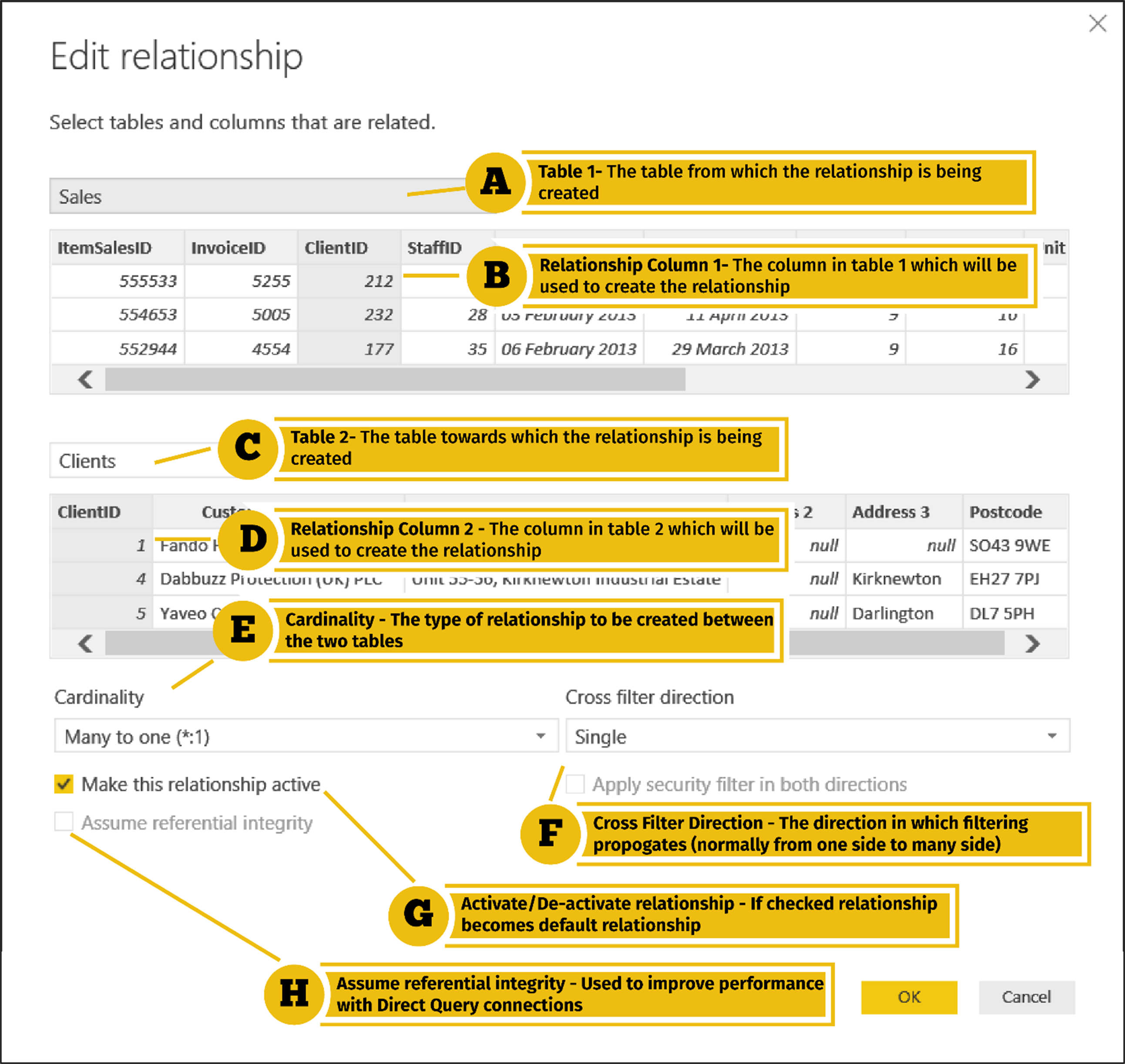
A: Table 1 (The “From” Table)

This is the table from which the relationship is being created. The table you choose as the first drop-down will determine the type of relationship you will create.

B: Relationship Column 1

This is the column in table 1 for which matching values will exist in table 2.

C: Table 2 (The “To” Table)

This is the table to which the relationship is being created.

D: Relationship Column 2

This is the column in table 2 for which matching values will exist in table 1.

E: Cardinality

Cardinality sets the type of relationship that you wish to create between the two tables. The options are: many-to-one/one-to-many, one-to-one and many-to-many. In Power Pivot, the cardinality option does not apply since all relationships have to be many-to-one/one-to-many.

Many to One (a.k.a. One to Many)

This is the default relationship for data modelling in Power BI and the only available option in Power Pivot. The table on the Many side of the relationship is normally a fact table containing many repetitions in the match column (the column used to link the two tables). The table on the one side is normally a dimension table which acts as a lookup table and cannot contain repeating values in the match column.

In the above Power BI and Power Pivot illustrations, we can see that Sales is the many table and Clients is the one. The ClientID column, in both tables, is the column has been used to create the many-to-one relationship, which is the same as a one-to-many relationship, if you look at it from the other point of view; in other words, if we reversed the table selection.

One to One

One to one relationships are hardly ever used. They tend to be used mainly in security scenarios; thus, if you have information which was sensitive, you might place it into a separate table and then you could use a feature of like row-level security to lock that table completely from one set of users.

Many to Many

In some more complex models, containing many tables, you may sometimes need to link two tables using a column which has repeating values in both tables. In these scenarios, Power BI allows you to create a many-to-many relationship.

Data Cardinality

It is worth noting that the word “cardinality” is also used in the context of data: the cardinality of a table column is the number of distinct values it contains, relative to the number of rows. A relatively high number of distinct values implies a high cardinality and, in the Power BI data model, requires more memory. This often becomes an important issue when creating calculated columns: columns with low cardinality have less of a negative impact on storage and performance than those with high cardinality.

F. Cross Filter Direction

Single

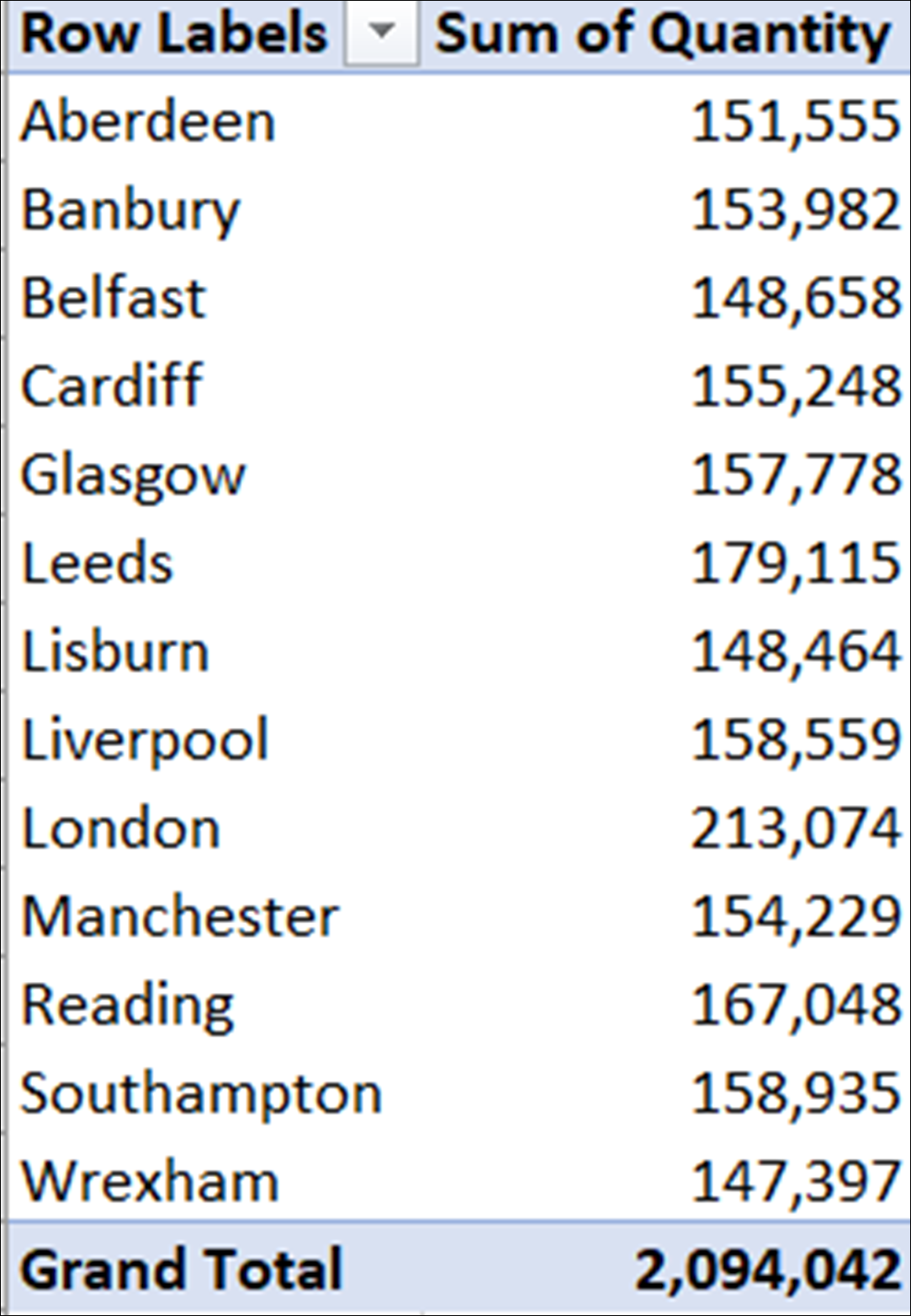
The filter direction of a relationship is the direction in which filtering can occur when using the values in a column of one table to filter data in the related table. In Excel, and by default in Power BI, the cross filter direction is from the one table to the many table; from the dimension table to the fact table. Thus, in the example shown in our illustration, we could use the Branch column in the Staff table to filter the Quantity Column in the Sales table by creating the pivot table shown below.

When the cross filter direction is set to single, the filter context always propagates from the one side of the relationship to the many. However, there may be times, in a data model, when you want to display filtering in the other direction; from the many side to the one side of the relationship.

Both

It is not usually the case that we want to filter from a fact table to a dimension table. The most common scenario is where we want to filter data in a dimension table using another dimension table and travelling via the fact table. The following illustration provides an example.

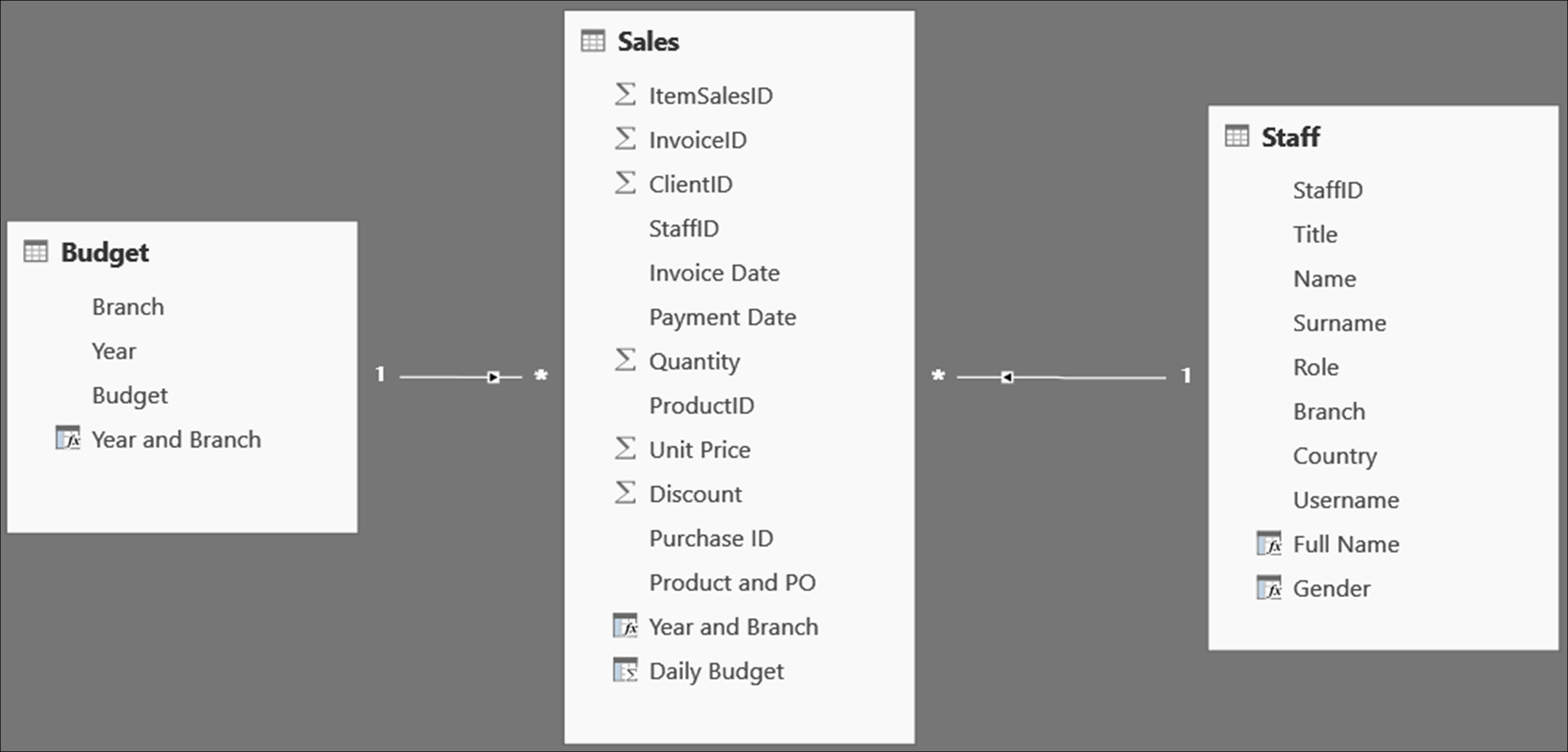
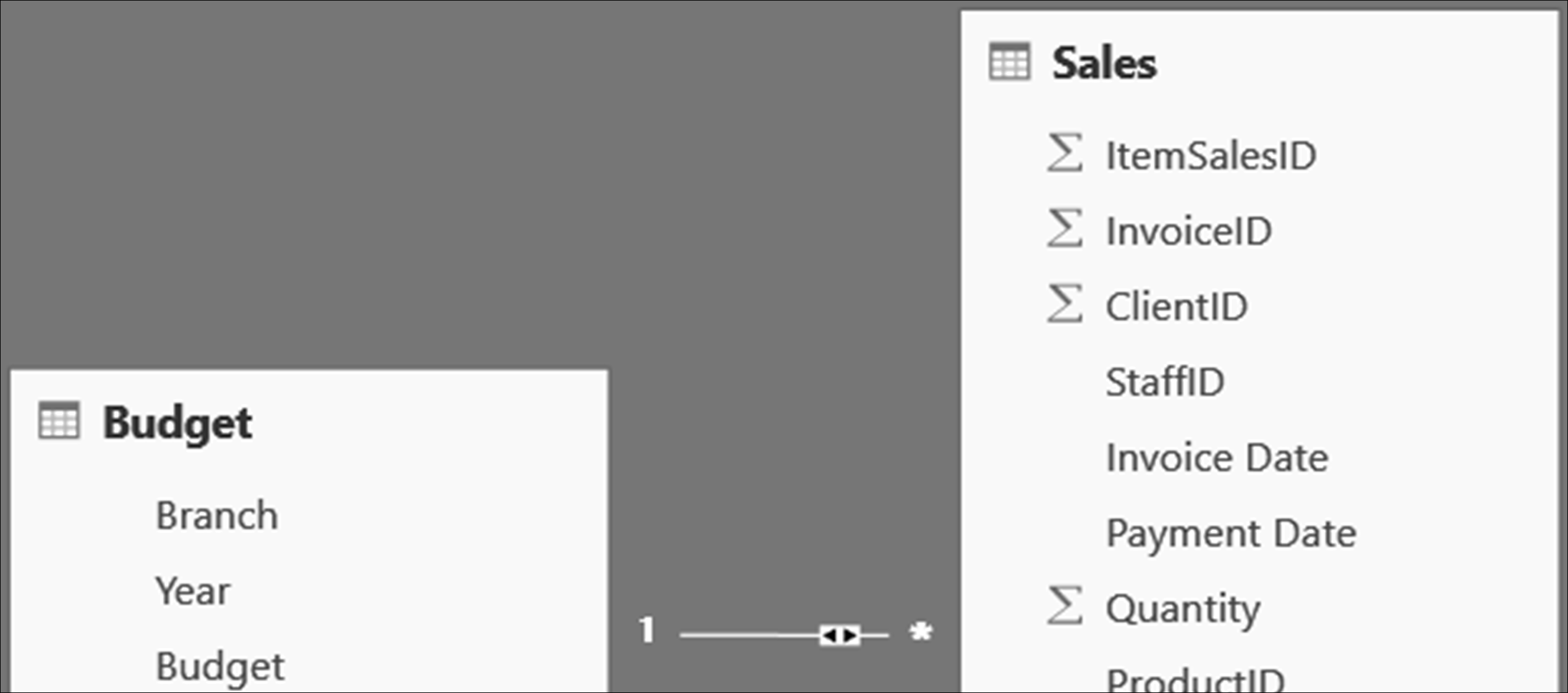
Our fact table is Sales and Staff and Budget are dimension tables linked to it. Staff is linked to Sales via the StaffID; and since each transaction in Sales has a StaffID to identify the seller, Staff and Sales have the same granularity; which means that we can use staff to filter Sales at the transactional level.

What if we wanted to aggregate Sales revenue by year and compare it with the annual budget/target set for each branch. We would need to filter both revenue and budget using the Branch column in the Staff table. However, the Budget table which is on the one side of its relationship with the Sales table. Therefore, to navigate from Staff to Budget, we go, first, from Staff to Sales (one to many; so, no problem), then from Sales to Budget (many to one; hence problematic, since no filtering can take place).

This is an example of where we can achieve the desired result by changing the Cross filter direction setting in the Edit Relationship dialog to Both.

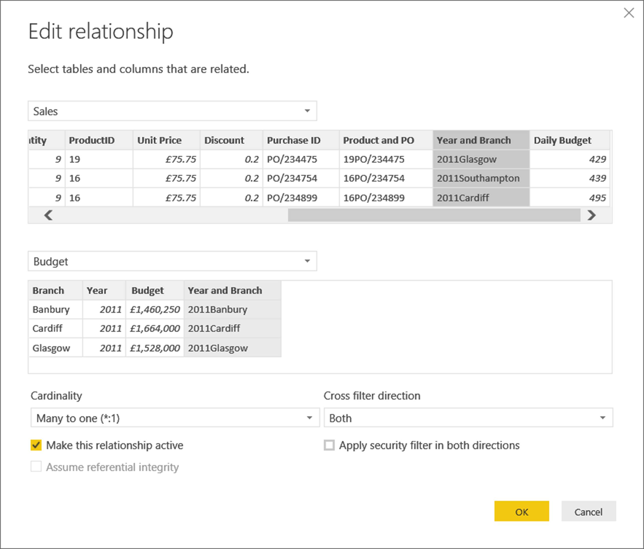
Once this change has been made, a bi-directional arrow is displayed on the line representing the relationship between the two tables.

We can then use any field in the Staff table to filter the information in the Budget table. Thus, for example, in the following illustration, each gauge is filtered to show a comparison of actual vs budget sales for a single country.

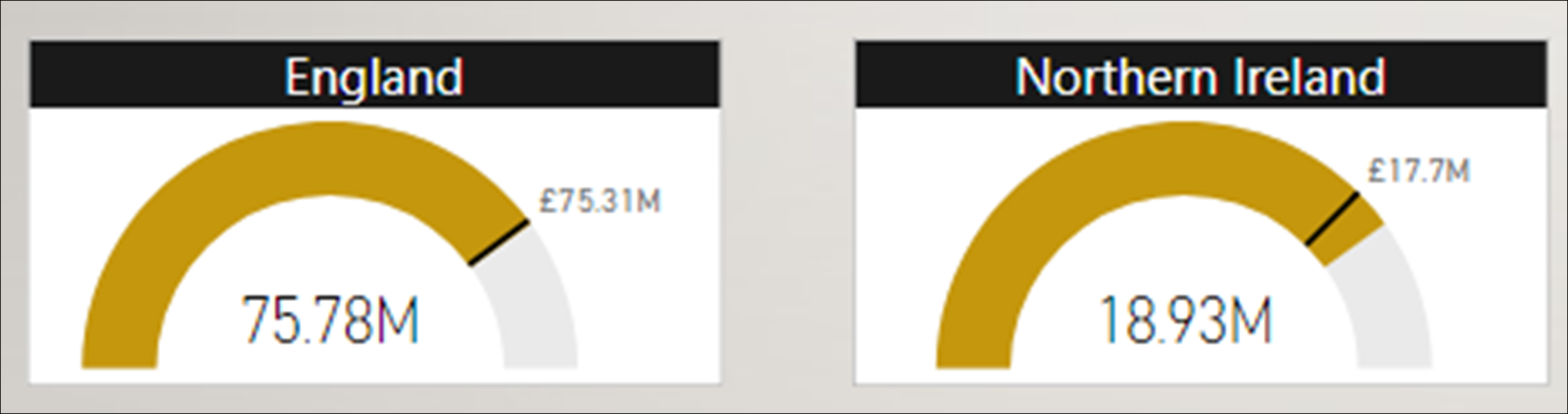
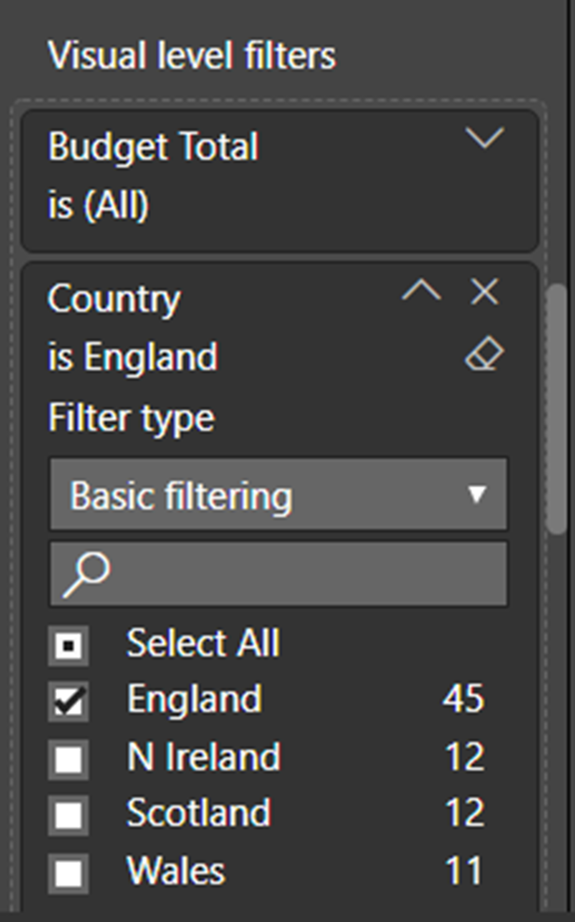
This is achieved by applying a visual level filter to the Country column in the Staff table which, because of the cross-filter direction is set to Both, propagates to the Budget table. Setting the cross-filter direction to both in a relationship has significant implications for performance and this feature should only be used when working with simple data models, if at all.

G: Active and Inactive Relationship

In both Power BI and Power Pivot, it is possible to create more than one relationship between the same tables. However, only one of these relationships can be active. The active relationship is the one which will enable the use of columns from both two related tables when building your report. However, the inactive relationship(s) can be referenced when creating DAX calculations by using the USERELATIONSHIP function.

The most common scenario is where you need to analyse the same information in a fact table but focus on different dates. For example, in the following illustration, we have a fact table containing information on sales leads. The Leads table is linked to a Calendar table which has a date column. The active link between the two tables is from Calendar[Date] to Leads[Sale Date].

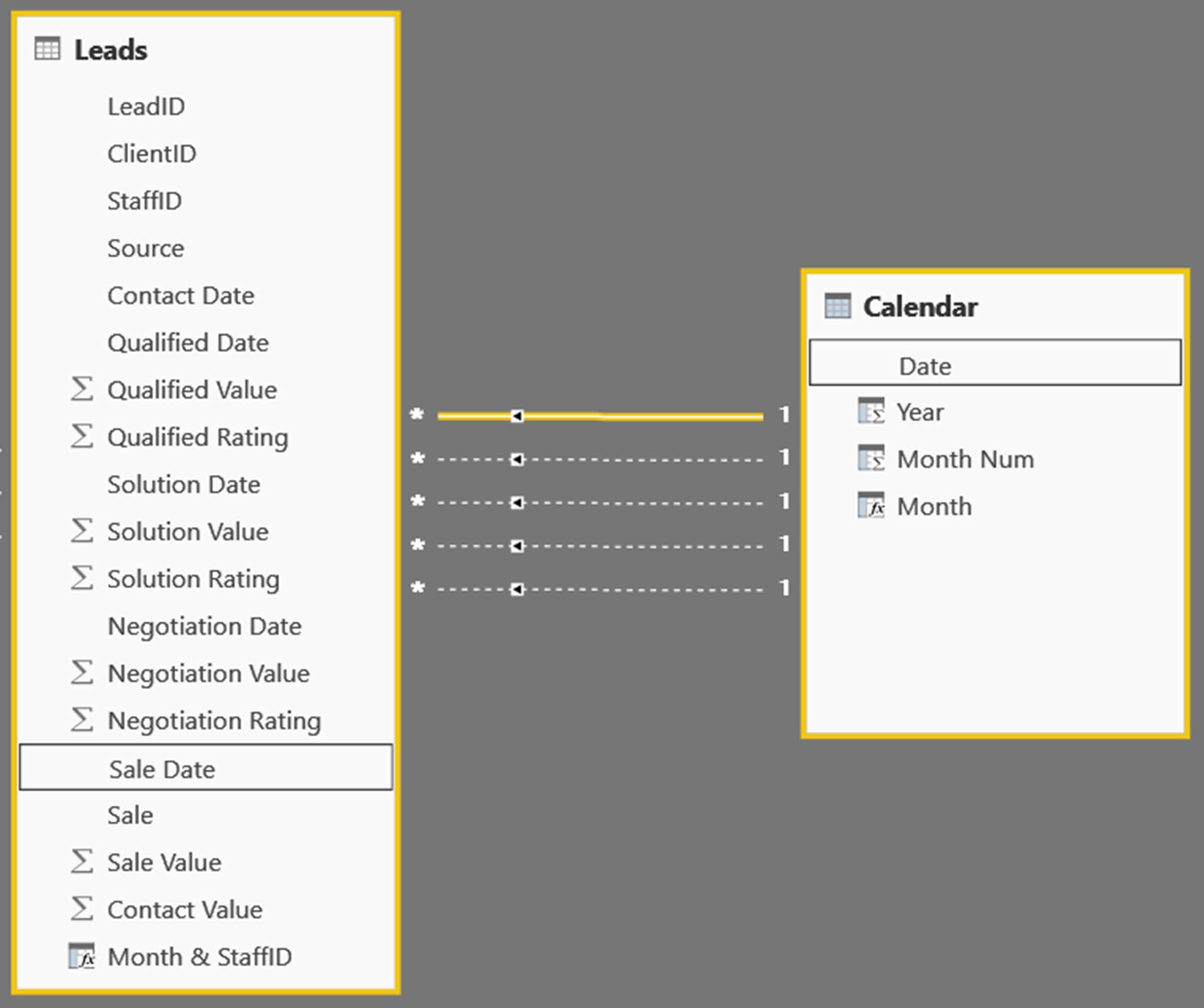
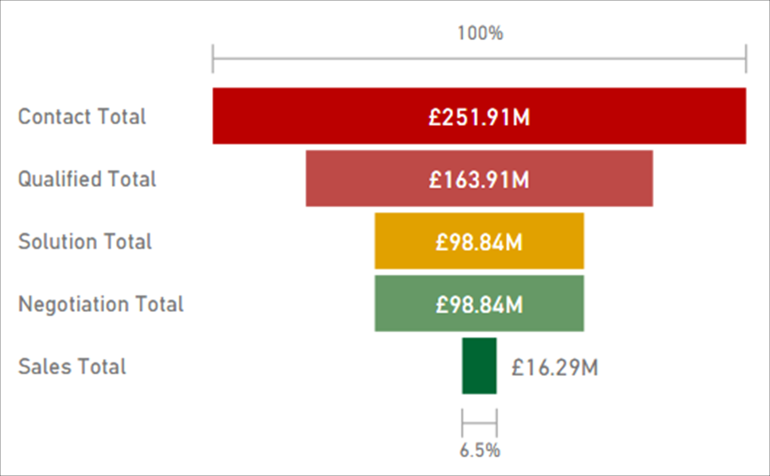
However, the Leads table contains four other significant dates: Contact Date, Qualified Date, Negotiation Date and Solution Date. To create our report, we need to focus on all five dates in the Leads table in turn. This is achieved by creating a total of five relationships between the two tables; with the relationship to Leads[Sales Date] active and the relationships to each of the other four inactive.

We need to calculate the monetary value of leads at all five stages at any given point in time.

To do this, we use a calculation which includes the USERELATIONSHIP function, when necessary, to activate the appropriate inactive relationship.

The calculation for the Sales total is straightforward, since Leads[Sales Date] to Calender[Date] is the active relationship.

Sales Total = SUM(Leads[Sale Value])

For the other calculations, we need to combine the CALCULATE and USERELATIONSHIP functions. For example, here is the formula for calcuting the Contact Total.

CALCULATE(

SUM(Leads[Contact Value]),

USERELATIONSHIP(

Leads[Contact Date],

‘Calendar'[Date]

)

)

 

H: Assume Referential Integrity

Unless you are using a DirectQuery connection, the Assume referential integrity option will be greyed out since this setting is designed to optimize the execution of queries against the database server. The technique it uses to achieve improvements if to use INNER JOIN, rather than OUTER JOIN, statements when executing queries.

For the Assume referential integrity setting to work properly, the following criteria must both be satisfied.

1.      The match column in the table on the many side of the relationship must not contain any null values.

2.      Each value in the match column in the table on the many side of the relationship must exist in the match column of the table on the one side.